Danylo Malyuta Research Works

The Sequential Convex Programming (SCP) Toolbox provides a suite of fast nonlinear optimal control algorithms for solving nonconvex trajectory generation tasks. These algorithms have been applied on problems for organizations such as NASA, SpaceX, Blue Origin, and Masten Space Systems. This post shows you how to get started with the SCP Toolbox by solving a simple obstacle avoidance problem for Dubin’s car model.

The SCP Toolbox is the result of a comprehensive tutorial paper that recently appeared in preprint. The paper covers the complete algorithmic and practical details of the low-level solvers that power the SCP Toolbox. In this post, I will just scratch the surface by providing a simple and concrete implementation of a trajectory generation problem. Keep in mind that this example does not reveal the full generality of the toolbox. If you are interested to learn more about SCP algorithms, I would really recommend that you supplement reading this post with the tutorial paper.

Purpose of the SCP Toolbox

The goal of the SCP Toolbox is to solve nonconvex optimal control problems of the following form:

This is known as a “template” optimal control problem because it defines a whole family of problems that can be solved by the SCP Toolbox. Note that the SCP Toolbox is capable of solving much more general problems as described in the previously mentioned tutorial paper. To keep this introductory post reasonably simple and to-the-point, I’ll only talk explicitly about problems of the form (??)–(??).

Let’s define the elements of this optimal control problem. The vectors , , and represent the state, input, and other “static” (in other words, time-independent) parameters. The function is the running and has to be convex. The vector function defines the path constraints, which can be nonconvex. Finally, the vector functions and denote the initial and terminal boundary conditions, which can also be nonconvex. Importantly, note that the trajectory evolves on a “normalized” time interval . This means that the user has to convert their problem’s “absolute” time to this normalized time convention. We will discuss this nuance explicitly when it comes to implementing the Dubin’s car problem.

Why Another Toolbox?

The SCP Toolbox joins a growing family of tools for solving nonconvex trajectory problems. These include TrajectoryOptimization.jl, Crocoddyl, OCS2, COSMO.jl, CasADi, and GPOPS-II. All of these tools solve some close or distance relative of the optimal control problem (??)-(??). Some of the tools target a real-time implementation (such as OCS2) while others are oriented towards an accurate but not real-time solution (such as GPOPS-II). Perhaps even more importantly, tools like GPOPS-II implement algorithms that are generally not aimed at real-time performance, while tools like TrajectoryOptimization.jl implement algorithms that can perform in real-time using an optimized implemenetation in a compiled language like C++.

The contribution of the SCP Toolbox is to provide a high-level parser-solver interface for a suite of promising new algorithms that are not accessible using existing tools. These algorithms are:

Lossless convexification (also known as LCvx, see the paper by Acikmese and Ploen, 2007).
Successive convexification (also known as SCvx, see the paper by Mao et al., 2019).
Penalized Trust Region method (also known as PTR, see the paper by Szmuk et al., 2019).
GuSTO, see the paper by Bonalli et al., 2019.

Under the hood these algorithms use some user-selected convex optimizer, for example an Interior Point Method-based solver like ECOS. LCvx is a “vanilla” convex optimization algorithm in the sense that the solver is called either once or some pre-determined (small) number of times¹¹The LCvx algorithm is quite different to the other three algorithms, which are SCP methods. Hence it sits a little awkwardly in an “SCP Toolbox”, but it is included anyway due to being part of the tutorial paper from which the SCP Toolbox originated. Just keep in mind that the descriptions in this post apply to the SCP algorithms, while LCvx kind of “sits apart” from that code (for example, the LCvx examples do not use the SCP “parser interface” discussed in this post). . The latter three algorithms are known as SCP methods, and they call the optimizer as part of a trust region optimization method. All four algorithms are capable of real-time performance, as demonstrated in Scharf et al., 2017, Dueri et al., 2017, and Reynolds et al., 2020. While the SCP Toolbox does solve problems quickly (on the order of seconds), it is first and foremost aimed at providing a generic, clean, and transparent implementation of the algorithms. Real-time implementations, unfortunately, tend to be terse and non-generic because they exploit specific problem structure. Therefore the SCP Toolbox trades some performance in favor of clarity and generality.

The theoretical guarantees and computational speed offered by convex optimization have made LCvx and SCP algorithms popular in both research and industry circles. LCvx, SCvx, and PTR have all been used in projects for NASA and Masten Space Systems, resulting in Xombie rocket flight tests and a Blue Origin experimental flight. The algorithms were also applied independently to research problems relevant for SpaceX rockets, such as the Starship landing flip maneuver. In robotics, all three SCP methods were used to control quadrotors and microgravity flying assistant robots. To summarize:

The purpose of releasing the SCP Toolbox is to provide public implementations of lossless convexification and sequential convex programming algorithms that have had marked success in modern nonconvex trajectory research and development.

Installation

First things first, I will assume the following things about your computer:

You are running Ubuntu 20.04
You have Julia 1.6.1 installed

If something doesn’t work, it is likely due to the above criteria not being met. If you cannot resolve an issue, please reach out to me.

Let’s begin by downloading the SCP Toolbox from its GitHub repository. Note that I link to the jgcd branch intentionally, since this branch contains the latest code from the recent JGCD paper. In the near future, this branch will be merged to master, so stay tuned. For simplicity, I’ll work in the /tmp/ directory, but you may choose any directory you like.

$ cd /tmp/
$ git clone https://github.com/dmalyuta/scp_traj_opt
$ cd scp_traj_opt
$ git checkout jgcd

Congratulations! You now have the SCP Toolbox on your computer. In the next section, we will discuss the file structure of the toolbox.

File Structure

If you navigate to /tmp/scp_traj_opt/ and run tree -L 1 then you will see the following file structure (I am only showing the folders):

.
├── solvers
├── parser
├── utils
├── examples
├── test
└── figures

You should typically not have to touch any of these folders. However, to help you work with the toolbox, it is instructive to describe the purpose of each folder:

The solvers/ directory contains the code of the low-level algorithms that I mentioned previously: SCvx, PTR, and so on. These solvers are generic in the sense that they expect optimal control problems to be defined using some “obscure” functions and matrices… not fun. A version of this generic problem was given above by (??)–(??). As a user, you want to specify problem in a higher-level code, which is where the next directory comes into play.
The parser/ directory contains code for the parser interface. The SCP Toolbox makes the reasonable assumption that as a user, your focus is on modeling and solving actual problems, not on developing the underlying algorithm that carries out the solution. Hence, code in parser/ implements a kind of front-end interface that allows you to specify your nonconvex trajectory generation problem. This will be communicated behind the scenes to the underlying solvers in solvers/, and you won’t have to do any of that “ugly” legwork.
The utils/ directory contains general code for common functions and objects that are used throughout the rest of the code. Hence you will find here a quaternion object, a bunch of geometric objects such as sets, interpolatable continuous-time trajectories, plotting functions, etc.
The examples/ directory contains solved examples of nonconvex trajectory generation problems. Each example has its own folder. For instance, the SpaceX Starship flip maneuver is located in examples/src/starship_flip/. You can think of these examples as unit tests for the SCP Toolbox that confirm that the rest of the code works as intended. They are also there for you to learn from to implement your own problems. However, examples/ is not where you should be implementing your own problems. In fact, this post is all about teaching you where and how to implement your problem correctly!

One other important thing about the examples. The reason that the jgcd branch has not yet been merged to master is because the examples in freeflyer/, quadrotor/, and rendezvous_planar/ have not yet been updated to the latest versions of the solver and parser code. The latest versions broke some of the backwards compatibility, hence the issue. In all the other working example folders, you will find the following file structure:
```
.
├── parameters.jl
├── definition.jl
├── plots.jl
└── tests.jl
```
In the same order as above, these files implement: the problem data structures, the problem definition functions (by using the parser code in parser/), the results plotting functions, and the unit test functions for solving an instance of the problem.
The tests/ directory contains a single test file that runs all of the unit tests – in other words, all the examples from the examples/ directory.
The figures/ directory should currently be empty except for a .gitkeep file. The results plots that are generated by the examples are placed in this directory as PDF files.

Okay, so now you know the lay of the land inside /tmp/scp_traj_opt/. Like I said above, you should not be editing this directory²²Unless you are developing your own solver or parser code and want to submit a pull request… in which case thank you and I’d like to buy you dinner. ! This leaves a question – where should you implement your own problems, and how are you to interface with the SCP Toolbox directory? This is covered in the next section.

Implementing Your Own Problem

At this point we have the SCP Toolbox available in the /tmp/scp_traj_opt/ directory. To implement your own problem, let’s talk a little bit about how Julia code is structured. Code is generally divided into packages. These are standard file structures for defining code modules (namespaces, roughly speaking), test scripts, and so on. The SCP Toolbox implements four packages³³Technically speaking these are “subpackages”, because the SCP Toolbox is itself a package. But this technicality doesn’t really matter for us. :

The Solvers package, which is implemented in the toolbox solvers/ directory.
The Parser package, which is implemented in the toolbox parser/ directory.
The Utils package, which is implemented in the toolbox utils/ directory.
The Examples package, which is implemented in the toolbox examples/ directory.

To implement your own problem, you need to do two things (at least this has been my personal workflow – once you get this to work, feel free to explore workflows that work better for you):

Create your own (new) package that holds your problem code.
Import the Solvers and Parser packages at the bare minimum, and usually also the Utils package because it provides helper functions for math, plotting, etc.

Let’s begin with the first step. If you don’t care for the details, I have actually created a GitHub repository that you may clone and that contains all of the code that we are about to write. However, I do recommend that you follow these steps manually at least once. I’ll create the package in the /tmp/scp_new_problem/ directory. Begin by navigating into /tmp/ and starting Julia:

$ cd /tmp
$ julia

You should now see the Julia read-eval-print loop (REPL). Each prompt line starts with julia>. If you type ] then you should see the package manager prompt ((@v1.6) pkg>), from which you can exit using backspace. Similarly you can type ; to enter shell mode (Bash in my case, and the prompt looks like shell>). Look out for these prompts as you follow along. Ready to create a new package for solving Dubin’s car problem? Let’s go.

(@v1.6) pkg> generate scp_new_problem
shell> cd scp_new_problem
(@v1.6) pkg> activate .
(scp_new_problem) pkg> dev ../scp_traj_opt/solvers/
(scp_new_problem) pkg> dev ../scp_traj_opt/parser/
(scp_new_problem) pkg> dev ../scp_traj_opt/utils/
(scp_new_problem) pkg> precompile

Note above the changes in the left-hand side prompt. Importantly, after the activate command the prompt changed to scp_new_problem to indicate that we are now working inside the new package’s environment. Keep this REPL open, we will come back to it shortly after editing some files.

To briefly describe the steps taken above, we first generate a new empty package. Next, we switch to the package’s directory and activate it. This switches the context for the subsequent commands from the “global” Julia environment to that of the new package. Next, the sequence of dev commands make the new package dependent on the SCP Toolbox packages that we mentioned above. Finally, the precompile step performs ahead-of-time compilation of the new package and its dependencies. This can save some time later when our code is executed (Julia tends to compile code just-in-time).

If you run the tree command line application inside /tmp/scp_new_problem/, you should see the following file structure:

.
├── Manifest.toml
├── Project.toml
└── src
    └── scp_new_problem.jl

The src/ folder is where you will implement your problem code. Let’s begin by changing the contents of the auto-generated file scp_new_problem.jl to the following code:

1
2
3
4
5
6
7
module scp_new_problem
include("./my_problem.jl")
end # module

using .scp_new_problem

scp_new_problem.solve()

Let’s also create a new file my_problem.jl in the src/ directory, and populate it with the following initial code:

1
2
3
4
5
6
7
8
9
10
11
12
13
14
15
16
using Solvers
using Parser
using Utils

using LinearAlgebra
using ECOS
using PyPlot
using Colors
using Printf

export solve

function solve()
    @printf("Problem code goes here...")
    return 0
end

Lines 1-3 import the SCP Toolbox packages that we mentioned earlier. This gives you access to the gamut of functionality of the SCP Toolbox for solving nonconvex trajectory generation problems. Lines 5-9 import other standard packages that we will make use of later (for example, the Printf package provides macros for C-style print statements via @printf). Line 11 exports the solve() function from the module. This function is where we will define and solve the Dubin’s car trajectory generation problem using the SCP Toolbox parser interface. From now on, because this is not a Julia language tutorial, I will assume that you have a working knowledge of Julia and I’ll stop commenting too much on the Julia language-specific features.

Let’s now return to the Julia REPL that we opened previously. Remember the state in which we left the REPL: we activated the scp_new_problem package, and the REPL was opened inside the /tmp/scp_new_problem/ directory. Now execute the following commands:

shell> cd src/
julia> include("scp_new_problem.jl");

If you see “Problem code goes here...” printed out, then congratulations! You have successfully loaded the relevant SCP Toolbox packages and executed the solve() function, which printed the placeholder statement. In the next section, we will populate the solve() function with the definition of the Dubin’s car obstacle avoidance problem, and solve it using the PTR algorithm.

Like I mentioned previously, note that I have made the /tmp/scp_new_problem/ directory available for download through GitHub. You can, for instance, clone this repository for each new trajectory problem that you want to solve. If you are more Julia savvy, you can also work on multiple problems at once by continuing to create more files and complex structures inside /tmp/scp_new_problem/.

One more thing is worth mentioning about the GitHub repository. Once you download it and start a new REPL, you will have to use the activate command in order to switch Julia’s context to the scp_new_problem package before you can run any code. For example, suppose that you cloned the repository into DIR and that you have a terminal shell open inside of DIR/src/ (the source file directory). When you start Julia using the shell’s julia, the REPL will be automatically opened in the DIR/src/ directory. You can then activate the scp_new_problem package using:

(@v1.6) pkg> activate ..

You will see the prompt change to (scp_new_problem) pkg> after this command. Note that we are using .. instead of . like before. This is because the REPL is inside the src/ directory, and package activation requires pointing to the directory that contains the Project.toml file which is located in the parent directory of src/.

Dubin’s Car Problem

I will now walk through an implementation of the solve() function from the last section. The goal is to solve an obstacle avoidance trajectory problem using Dubin’s car model. To begin, let’s write down the mathematical formulation of the problem. The setup can be visualized as shown in Figure 1.

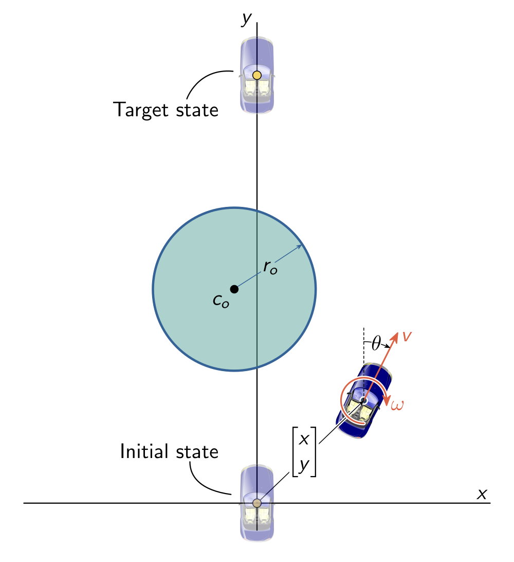
Figure 1. Visualization of the obstacle avoidance trajectory generation problem using Dubin's car model.

Dubin’s car is a simple agent that moves in a 2D plane. For trajectory generation we get to decide the forward velocity and the turn rate . Using these control inputs, we want to steer the car from an initial to a final position while avoiding the green circular obstacle. Long story short, this results in the following optimal control problem:

Let’s discuss this problem a bit. Equations (??)–(??) are the equations of motion (also known as the dynamics) for Dubin’s car. The SCP Toolbox computes dynamically feasible trajectories, and the equations of motion define what exactly “dynamic feasibility” means. Equation (??) defines the nonconvex obstacle avoidance constraint. Here, the obstacle is a circle of radius meters that is centered at the position . Finally, equations (??) and (??) define the boundary conditions. The car starts at the origin facing north, and should end up 2 meters along the axis facing the same direction. Note that we have confined the optimization to look for a 3 second trajectory that minimizes the control usage according to the cost function in equation (??). Intuitively, we are looking for a “mild” trajectory that drives the car to its destination “with least effort”.

Now that we have an optimal control problem that specifies the desired trajectory, it is time to plug it into the SCP Toolbox. We do this by using the previously mentioned parser interface to convert equations (??)–(??) into the template form (??)–(??).

Optimal Control Problem Implementation

The purpose of the SCP Toolbox parser in /tmp/scp_traj_opt/parser/ is to provide a set of high-level functions for defining (??)–(??) given your application-specific optimal control problem (??)–(??). Going back to the solve() function from the last section, we will now replace the @printf placeholder with the parser code for our Dubin’s car trajectory problem. Begin by changing the solve() function to the following:

1
2
3
4
5
function solve()
    pbm = TrajectoryProblem(nothing)
    problem_set_dims!(pbm, 3, 2, 1)
    # More code...
end

On line 2 we initialize the optimal control problem as a TrajectoryProblem structure, which is defined in the Parser package of the SCP Toolbox. The constructor for TrajectoryProblem accepts one generic argument that can hold problem-specific data, such as a custom dictionary or a structure that is totally up to you to define. Dubin’s car problem is pretty simple so we will stick to global variables for this tutorial – hence we will pass nothing here. For examples where a custom structure is passed to the TrajectoryProblem constructor, see the aforementioned examples/ directory of the SCP Toolbox.

On line 3, we begin by defining the state, input, and parameter dimensions – in other words, the values of , , and from equations (??)–(??). For Dubin’s car we have three states (), two inputs (), and no static parameters that need to be optimized. However, the SCP Toolbox is currently limited to due to implementation edge cases that need to be handled explicitly when either value becomes zero. Hence we have to set even though mathematically we know that . This means that we will need to stay cognizant of the fact that a one-dimensional “dummy” parameter vector will appear in the underlying optimal control problem, even though none of our constraints nor cost end up using it.

Quick sidenote. To not have to keep writing the complete solve() function definition every time, the code snippets that I provide from now on will be replace the # More code... comment on line 4 above.

The low-level algorithms of the SCP Toolbox require an initial trajectory guess. As discussed in the associated tutorial paper, SCP algorithms have the nice property that this guess can typically be very simple. In the case of Dubin’s car, we use a straight-line trajectory from start to finish as our guess (even though this trajectory is infeasible with respect to the obstacle constraint). This is done using the code below.

1
2
3
4
5
6
7
8
9
10
_x0 = [0; 0; 0] # Initial state
_xf = [0; 2; 0] # Terminal state
problem_set_guess!(
    pbm, (N, pbm) -> begin
        x = straightline_interpolate(_x0, _xf, N)
        idle = zeros(pbm.nu)
        u = straightline_interpolate(idle, idle, N)
        p = zeros(pbm.np)
        return x, u, p
    end)

As you can see, we use the function problem_set_guess! that is provided by the parser to set the initial guess. This accepts an anonymous function whose argument N corresponds to the number of discrete time nodes in the trajectory. On line 5 we perform a straight-line interpolation for the state between the initial and terminal states. We do the same on line 7 for the input, for which we use a “zero velocity, zero turn rate” initial guess. The parameter vector is also set to zero on line 8. Remember that although we do not have any parameters in the mathematical problem, we had to set the parameter to a dimesion of due to the current limitations of how the SCP Toolbox works. Therefore, we use zeros(pbm.np) in order to define a zero vector of length one for the parameter guess.

Note that in the code above we are using two “global” variables _x0 and _xf that define the initial and final conditions according to (??) and (??). Like I mentioned above, we could have also opted for storing these variables in a dictionary or a structure that we then pass to the TrajectoryProblem constructor. Here is an example code sketch:

1
2
3
4
5
6
7
8
9
data = Dict(:x0 => [0; 0; 0], :xf => [0; 2; 0])
pbm = TrajectoryProblem(data)
# More code ...
problem_set_guess!(
    pbm, (N, pbm) -> begin
        data = pbm.mdl
        x = straightline_interpolate(data[:x0], data[:xf], N)
        # More code ...
    end)

The next step is to translate the cost function (??) into its generic form (??). Again, we do this with the help of the parser:

1
2
problem_set_running_cost!(
    pbm, :ptr, (t, k, x, u, p, pbm) -> u'*u)

The parser function problem_set_running_cost! is responsible for defining the function from (??). Like before, this is done with a user-defined anonymous function that computes the running cost value. This function has to accept a bunch of different arguments, but for this example I’d like to focus on the only relevant argument u, which is the input vector value at the normalized time t. Previously we defined a two-dimensional input vector . Comparing this vector with equation (??), we realize that the running cost is quite simply the dot product . This is exactly what we enter on line 2 in the above code snippet.

Our next challenge is to define the equations of motion, also known as the dynamics. This amounts to translating the differential constraints (??)–(??) into the generic form (??). This is done using the parser as follows:

1
2
3
4
5
6
7
8
9
10
11
12
13
14
15
16
17
18
19
20
21
_tf = 3
problem_set_dynamics!(
    pbm,
    # f
    (t, k, x, u, p, pbm) ->
        [u[1]*sin(x[3]);
         u[1]*cos(x[3]);
         u[2]]*_tf,
    # df/dx
    (t, k, x, u, p, pbm) ->
        [0 0 u[1]*cos(x[3]);
         0 0 -u[1]*sin(x[3]);
         0 0 0]*_tf,
    # df/du
    (t, k, x, u, p, pbm) ->
        [sin(x[3]) 0;
         cos(x[3]) 0;
         0 1]*_tf,
    # df/dp
    (t, k, x, u, p, pbm) ->
        zeros(pbm.nx, pbm.np))

Evidently this step is a bit more complicated than what we’ve seen thus far. Four anonymous functions are defined: the first function defines in (??) and the remaining three functions define its Jacobians , , and . The Jacobians are needed because sequential convex programming works by linearizing nonconvex parts of the problem, and this linearization (which is a first-order Taylor series expansion) needs the Jacobian values. By defining the three-dimensional state vector as (please excuse the overloaded notation for the -position), we can write the dynamics (??)–(??) as follows:

There is one issue that remains, and this is the conversion between absolute and normalized time. Equation (??) is written in absolute time, which runs like the clock on your wall (if you have one). Recall that (??)–(??) is defined on normalized time, which invariably runs on the time interval. Let’s denote the normalized time by and the absolute time by . Let’s also generalize the Dubin’s car problem statement a bit and say that the trajectory we’re looking for runs on where is the “final time” (in our case, ). We hence have the relationship between absolute and normalized time, and we can use the chain rule to write:

Equation (??) reveals a simple relationship between the equations of motion expressed using the two “times”: to get the dynamics in normalized time, multiply the absolute time dynamics by . You can see that lines 6-8 exactly implement the original equations of motion (??) scaled in this way by . I’ll assume that you are familiar with differential calculus, so the remaining three anonymous functions for the Jacobians of should be self-explanatory.

Similar to the dynamics, we will now translate the nonconvex obstacle avoidance constraint (??) into its generic form (??). Using the parser, this looks as follows:

1
2
3
4
5
6
7
8
9
10
11
12
13
_ro = 0.35
_co = [-0.1; 1]
_carw = 0.1
problem_set_s!(
    pbm, :ptr,
    # s
    (t, k, x, u, p, pbm) -> [(_ro+_carw/2)^2-(x[1]-_co[1])^2-(x[2]-_co[2])^2],
    # ds/dx
    (t, k, x, u, p, pbm) -> collect([-2*(x[1]-_co[1]); -2*(x[2]-_co[2]); 0]'),
    # ds/du
    (t, k, x, u, p, pbm) -> zeros(1, pbm.nu),
    # ds/dp
    (t, k, x, u, p, pbm) -> zeros(1, pbm.np))

The parser function problem_set_s! works very similarly to the function problem_set_dynamics! that we used for the dynamics. Four anonymous functions are defined, this time for the function in (??) and its Jacobians , , and . It should be easy to relate the code snippet to (??). The first anonymous function simply writes the function as a one-dimensional vector. The other three anonymous functions compute the Jacobian using the standard differential calculus definition. Note that given , we have (in other words, a row vector), and similarly for the other Jacobians.

An interesting bit of trajectory engineering heuristics occurs on line 7, and it is worth mentioning. The physical car is not a point object, so a collision will occur if it approaches the obstacle too closely. We define the variable _carw to store the car body’s width. Then, we “inflate” the physical obstacle of radius meters by half of the car’s width. This results in an effective keep-out circular zone of radius meters. The car will no longer approach the obstacle too closely, and collisions will be avoided as long as the car’s motion is sufficiently tangential to the obstacle.

The last bit of code needed to fully define the optimal control problem is to convert the boundary conditions (??)–(??) to their generic form (??)–(??). The parser allows us to do this like so:

1
2
3
4
5
6
7
8
problem_set_bc!(
    pbm, :ic, # Initial condition
    (x, p, pbm) -> x-_x0,
    (x, p, pbm) -> I(pbm.nx))
problem_set_bc!(
    pbm, :tc,  # Terminal condition
    (x, p, pbm) -> x-_xf,
    (x, p, pbm) -> I(pbm.nx))

The function problem_set_bc! allows us to set both the initial conditions (when its second argument is :ic) and the terminal conditions (when its second argument is :tc). Two anonymous functions are passed: one defining the boundary condition function itself (either or ) and another defining its Jacobian with respect to the state (either or ). In the case where the functions also depend on the parameter vector , a third anonymous function has to be passed that defines the corresponding Jacobian. This is not the case for this simple problem, but you may check out the other examples in /tmp/scp_traj_opt/examples/src/ to see how that functionality works. Comparing (??) and (??) with the code snippet, we can see that the code is self-explanatory (the Jacobians in this case are the identity matrix, since the full state is being constrained at both endpoints).

Solver Setup

Congratulations, at this point we are done using the parser to convert the Dubin’s car optimal control problem (??)–(??) to the generic form (??)–(??). The next step is to define the solver algorithm parameters. This is done by populating the Parameters structure for one of the SCP solvers that is available in the toolbox (PTR, SCvx, of GuSTO). We will use the PTR solver, which is implemented in the file /tmp/scp_traj_opt/solvers/src/ptr.jl.

1
2
3
4
5
6
7
8
9
10
11
12
N, Nsub = 11, 10
iter_max = 30
disc_method = FOH
wvc, wtr = 1e3, 1e0
feas_tol = 5e-3
ε_abs, ε_rel = 1e-5, 1e-3
q_tr = Inf
q_exit = Inf
solver, options = ECOS, Dict("verbose"=>0)
pars = Solvers.PTR.Parameters(
    N, Nsub, iter_max, disc_method, wvc, wtr, ε_abs,
    ε_rel, feas_tol, q_tr, q_exit, solver, options)

Let’s go through the options step-by-step (note that some documentation on each option is provided in the comments of the Parameters structure):

N, Nsub: the first parameter defines the discretized trajectory’s number of temporal grid nodes, and the second parameter defines the number of steps used by the Runge-Kutta (RK4) algorithm to integrate “in between” the temporal grid nodes.
iter_max: the maximum number of SCP iterations.
disc_method: the temporal discretization method used. Currently FOH and IMPULSE are implemented. The first method linearly interpolates the input values in between the temporal grid nodes, while the second method assumes that the inputs are “impulsive” – in other words, each input is a scaled Dirac impulse that occurs at the discrete temporal nodes. Roughly speaking, I use FOH for control inputs that should be continuous, while IMPULSE was implemented specifically for optimizing spacecraft trajectories with pulse-fired reaction control system thrusters. The code is written generically enough to allow for more discretization methods to be implemented.
wvc, wtr: these are the virtual control and trust region penalty weights for the augmented cost function. See the tutorial paper for more information on these. These penalties are fundamental to SCP algorithms, but their discussion will take us too far away from the purposes of this tutorial.
feas_tol: this threshold governs how small the RK4 integration error across a single time interval must be in order to validate that a trajectory is dynamically feasible. Setting this to zero is unrealistic, since there will always be a tiny amount of numerical error.
ε_abs, ε_rel: these are the absolute and relative thresholds for the convergence stopping criterion. Again, I would suggest checking out the tutorial paper for more information.
q_tr: the type of norm used for the trust region constraint in the intermediate optimization subproblems that SCP generates. You have several options:
- 1: use the L1 “Taxicab” norm, in other words .
- 2: use the L2 “Eucledian” norm, in other words .
- 4: use the L2 norm squared, in other words .
- Inf: use the L-infinity “Maximum” norm, in other words . This is the norm that I’ve had most consistent success with, since it returns directly the value of the “largest” element in the vector (which I’m using as a placeholder here for whatever quantity).
q_exit: again a norm choice, with the same options, except this one is used for the stopping criterion.
solver: which convex solver do you want to use? Roughly speaking, as long as the solver can be called by the JuMP.jl library, you can put it here⁴⁴The caveat here is that the solver has to support the kinds of convex constraints that you are using in your optimal control problem. For example, if you use second-order cone constraints in combination with a quadratic problem solver, you’ll get an error during the solution process. .
options: a dictionary of options that the solver accepts. In the above code, I set a verbose flag to prevent the ECOS solver from printing out its solution process every time that it is called.

Congratulations, you’ve now “configured” the PTR solver and, believe it or not, it is ready to be used for Dubin’s car trajectory generation. So, are you ready to solve the problem? Here’s how you do it:

1
2
ptr_pbm = Solvers.PTR.create(pars, pbm)
sol, history = Solvers.PTR.solve(ptr_pbm)

The first line creates the problem. The function Solvers.PTR.create is defined by the PTR solver, and instantiates a ptr_pbm object based on two inputs. The argument pars specifies the PTR algorithm parameters that we just defined, while pbm specifies the optimal control problem that we defined using the parser functions (note how the first argument of all the problem_set_* functions from before was pbm – these functions were operating on the internals of the pbm object!).

The second line solves the optimal control problem, and returns the solution (sol) and a history of intermediate iterates of the algorithm (history). On my four-year-old Dell XPS 13 laptop, the whole solution process takes less than one second. The output in the Julia REPL should look something like this:

Results

k  | status   | vd    | vs    | vbc   | J         | ΔJ %  | Δx    | Δu    | Δp    | δ     | dyn | ηx    | ηu    | ηp
---+----------+-------+-------+-------+-----------+-------+-------+-------+-------+-------+-----+-------+-------+------
| OPTIMAL  | 3e-11 | 1e-01 | 1e-13 | 1.66e+01  |       | 3e-01 | 2e+00 | 0e+00 | 3e-01 | T   | 0.28  | 2.08  | 0.00
| OPTIMAL  | 3e-12 | 2e-12 | 2e-14 | 8.40e+00  | 49.35 | 1e+00 | 5e+00 | 0e+00 | 1e+00 | F   | 1.29  | 5.17  | 0.00
| OPTIMAL  | 8e-15 | 4e-16 | 5e-15 | 2.69e+00  | 67.91 | 8e-01 | 4e+00 | 0e+00 | 8e-01 | F   | 0.85  | 4.12  | 0.00
| OPTIMAL  | 2e-12 | 3e-13 | 3e-13 | 1.13e+00  | 58.12 | 1e-01 | 3e-01 | 0e+00 | 1e-01 | T   | 0.12  | 0.33  | 0.00
| OPTIMAL  | 5e-12 | 5e-13 | 5e-13 | 9.84e-01  | 12.76 | 1e-02 | 5e-02 | 0e+00 | 1e-02 | T   | 0.01  | 0.05  | 0.00
| OPTIMAL  | 4e-12 | 1e-12 | 4e-13 | 9.54e-01  | 3.06  | 3e-04 | 2e-03 | 0e+00 | 3e-04 | T   | 0.00  | 0.00  | 0.00
| OPTIMAL  | 3e-08 | 9e-09 | 1e-09 | 9.54e-01  | 0.08  | 7e-08 | 6e-08 | 0e+00 | 7e-08 | T   | 0.00  | 0.00  | 0.00

If this is roughly what you got on your computer (to within any small numerical error, perhaps), then great work! PTR just solved the Dubin’s car problem in 7 iterations, and the solution is stored in the sol and history variables. Before poring over some pretty results plots, it’s helpful to decypher what this progress table is telling us⁵⁵Note that each SCP solver has a slightly different progress table, based on the runtime variables that are relevant for the specific solver. :

k: the current iteration number.
status: the internal status of the convex optimizer (ECOS in the present case).
vd, vs, vbc: these give the L-infinity norms of the dynamics virtual control (vd) and the nonconvex constraint virtual buffers (vs for the path constraints (??), and vbc for the boundary conditions (??)–(??)). If the algorithm is converging, these values should become very small (of a “numerical error” magnitude, such as ).
J, ΔJ: these give the augmented cost function value and the percent change in this value relative to the previous iteration. The “augmented” cost function is a sum of the original cost function (??) and the virtual control and trust region penalty terms (see the tutorial paper for details). As the algorithm converges, these penalty terms become quasi-zero so J gradually starts to reflect the original cost function’s value. If you see positive values in the ΔJ column, it means that the cost function decreased relative to the last iteration. Since we seek to minimize the cost function, seeing positive values is good. However, it is normal if there are iterations where the cost function increases – this is simply part of the algorithm’s search for a locally optimal solution.
Δx, Δu, Δp: similar to vd, vs, and vbc, these values give the L-infinity norm deviations of the current solution’s state/input/parameter vectors from the previous solution. If the current iteration’s solution is very close to the last, these values will be small. Note that these values decrease as the iterations progress, which is indicative of the algorithm converging.
δ: this value measures the “distance” by which the current solution has moved away from the previous iteration’s solution. The measurement is done using a norm, and depends on the algorithm parameter q_exit from before. Note that this distance is given in terms of scaled state/input/parameter variables. I leave the details of variable scaling for the tutorial paper, since scaling is an important matter all by itself in the numerical optimization literature.
dyn: T signifies that the current solution is dynamically feasible, while F means that the numerically integrated trajectory does not sufficiently match the one output by the optimization, according to the feas_tol algorithm parameter.
ηx, ηu, ηp: these give the L-infinity norms of the state/input/parameter trust regions. As the algorithm converges, the trust regions shrink to zero, since the trust region size is penalized in the cost and it upper-bounds the amount by which the current solution is allowed to deviate from the previous iteration’s solution. Note how ηp is always zero, since we never actually use the “dummy” one-dimensional parameter vector (it is initialized to zero, and stays that way for the whole solution process).

We have now solved the Dubin’s car trajectory generation problem, and we understand how to read the progress table. It is time to generate some plots of the computed trajectory. This boils down to extracting the relevant data from sol and history and plotting it using your library of choice. Many examples are available already in the SCP Toolbox, and you can check them out in /tmp/scp_traj_opt/examples/src/. For this tutorial, let’s use PyPlot.jl to draw the Dubin car’s trajectory. There are many ways to do this, and in this tutorial I’ll do the following. First, let’s return the sol object from the solve() function by replacing return 0 with:

1
return sol

Then, in the scp_new_problem.jl file let’s replace scp_new_problem.solve() with:

1
2
solution = scp_new_problem.solve()
scp_new_problem.plot(solution)

Basically, we are taking the sol object, putting it into the solution object, and then passing that object to the plot function that we are going to dedicate to (you guessed it) plotting the trajectory. Then, back in the my_problem.jl file, create the plot() function:

1
2
3
4
5
6
export plot

function plot(sol)
    # Plotting code goes here
    return nothing
end

I won’t discuss the plotting code here, but you can find it in the GitHub repository. The code has little to do with the SCP Toolbox except familiarizing yourself with how the solution data is organized in the sol object. In particular, it is an SCPSolution structure implemented in /tmp/scp_traj_opt/solvers/src/scp.jl. Enough talk – here is the computed trajectory:

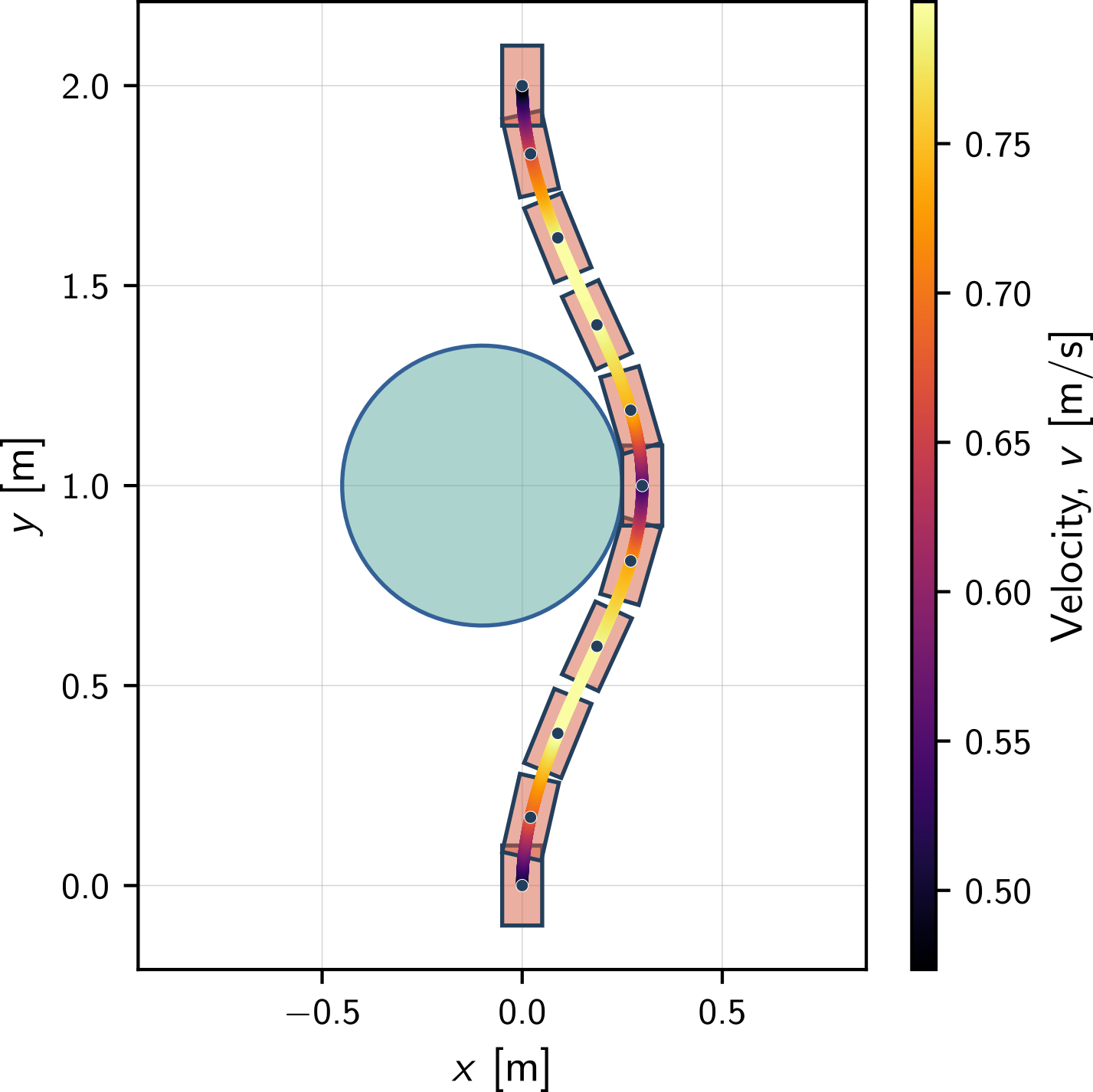
Figure 2. Dubin's car trajectory for a "small" obstacle radius of 0.35 meters.

We can see that the output is a smooth trajectory and quite predictable for a “minimum effort” cost function. Intuitively, the car “hugs” the obstacle to minimize the effort spent in driving around it. The velocity colormap shows that the car slows down while rounding the obstacle. Because the velocity is always positive, we conclude that the car is always driving forward.

Because we wrote the optimal control problem generically, let’s investigate what happens to the trajectory for a bigger obstacle. We do this simply by changing the _ro variable’s value to 0.8. This time, the PTR algorithm takes 20 iterations to converge, but the total solution time taken by the SCP Toolbox is still sub-second.

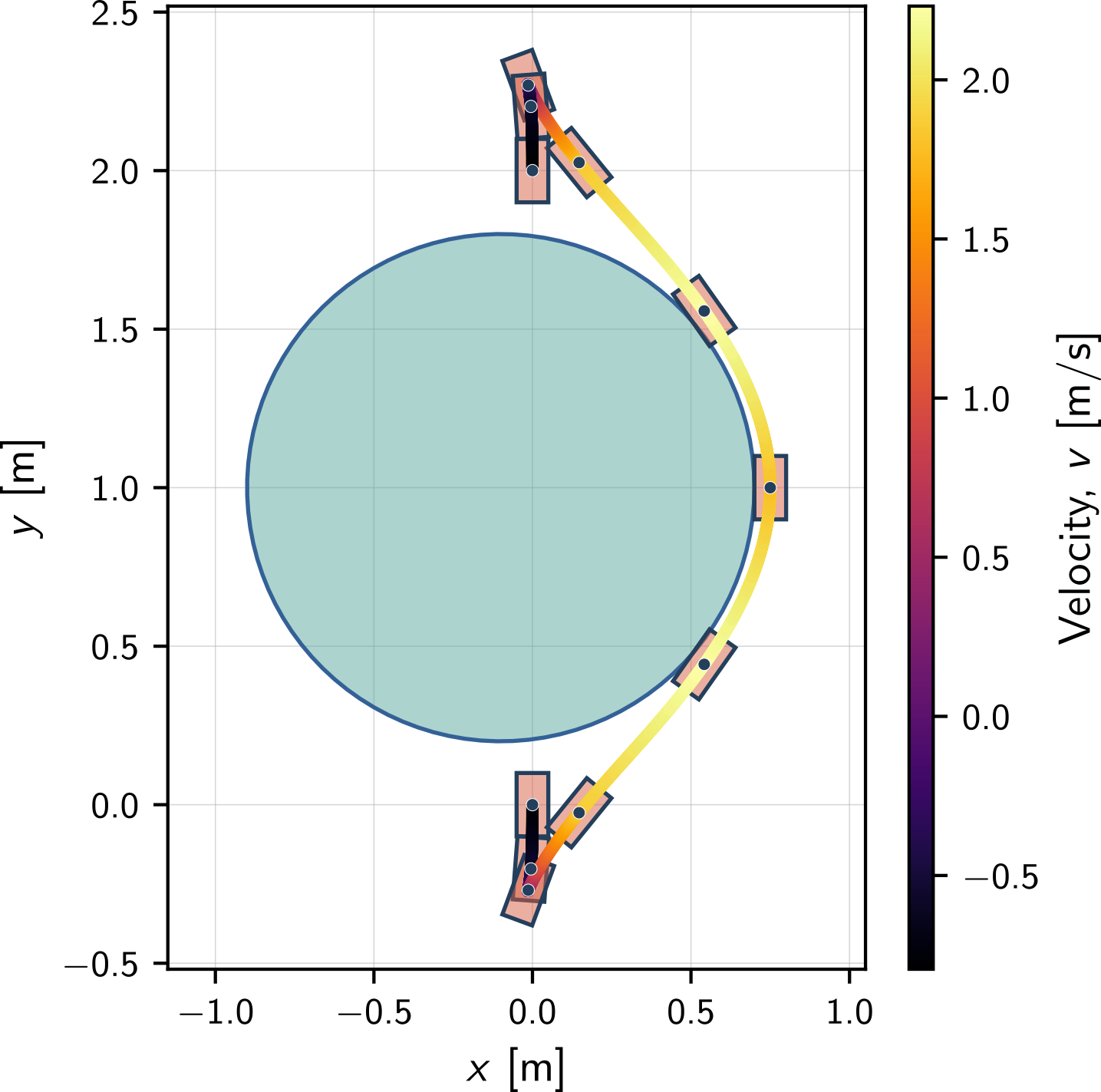
Figure 3. Dubin's car trajectory for a "big" obstacle radius of 0.8 meters.

Something very interesting has happened – without giving any new information to the optimization (remember, the initial guess is still just a straight line from start to finish), the car now decides to do a reversing maneuver and drive backwards in order to first back away from the large obstacle, and then to reverse park into the destination. I’d like to say that the optimization algorithm shows “creativity”, because this is a fundamentally different trajectory than the previous one, and certainly it is not close to what we provided as the initial guess. The SCP algorithm used the vehicle’s dynamics (??)–(??) in order to come up with a novel dynamically feasible trajectory. This is pretty exciting, and it is just one example of the kinds of nuanced tricks that optimization-based trajectory generation can teach us.

Conclusion

Hopefully this tutorial has shown you how to use the SCP Toolbox to solve a fairly simple, but nonconvex, trajectory generation problem for Dubin’s car. We also peeked under the hood and saw how the toolbox is organized, and developed a generic framework for how you can use the toolbox in your own personal projects. This amounts to creating a new Julia package that holds your trajectory generation problems, and placing that package alongside the SCP Toolbox. The Julia package that we created in this tutorial is available verbatim on GitHub for your future reference. It can serve as a template to quickly start implementing new and exciting problems.

Finally, I’d like to say a big thank you for taking the time to read this post. Happy problem solving!